As I promised in my last post, I will give two more examples of games, where it is better to be the weaker/less capable player.
The first game is three person Russian roulette: Three persons roll a dice to decide who is player A, B and C. First player A tries to shoot one of his opponents, if player B is still alive he tried to shot one of his opponents, then it is player C’s turn if he is still alive, after that it is player A’s turn and so on, until only one person is left. We assume that all shots are either lethal or a miss and we require all player to do their best at each shoot: you are not allowed to miss on purpose. If all three contestants have 100% chance of hitting on each shot, player A will kill one of B and C, and the survivor will kill player A. If A chooses his victim randomly (to be correct: with uniform distribution) then player B and C each have 50% chance of winning, and player A will die. However, if player B has only 99% chance of succeeding at a shot – and his opponents knows that – then player A will shoot player C, to get a 1% chance of surviving. Then player B has a 99% chance of winning. Similarly, if player C has 99% chance of succeeding on each shot, and A and B has 100%, then player C will win with probability 99%. Finally, consider the case where player A has 99% chance of hitting and the two others have 100%. If player A misses his first shot, he will be in the same situation as if he was player C, so he will win with probability 99%. If he hits in his first shot, the other player will hit him. Thus player A has 1%
This game has another “paradox”. If you are player A, you hope to miss your first shot. If we change the rules to allow the player to miss on purpose (and to avoid a stalemate, let’s stay that everyone dies if there are three misses in a row) the player with 99% chance of succeeding at each shot will survive with probability 99%, while each perfect shooter will only survive with a probability of 0.5%.
It might not be surprising that the weakest player can have an advantage in three person games: The two best compete against each other and then the weakest player can attack the survivor of the two strongest. I think the game from the last post was more surprising. Here two players play chicken, but one of the players, let’s call him player B, cannot turn the steering wheel. If player B could turn the steeling wheel, there would be two Nash equilibria, one where player A wins the most and one where player B wins the most. But when player B cannot swerve, the Nash equilibrium where A wins the most disappears, and we end up in the Nash equilibrium where B wins the most.
I find the next game even more surprising. This game also have two players, A and B with A being stronger that B, but now both A and B can “do the same to the environment” and player A can choose to use his strength against player B. The game is played by two pigs. They are trained separately to press a panel in one end of their sty to get food in a feeding bowl in the other end of the sty. We then put both pigs in the sty together. We assume that the dominant pig, A, can push B away from the feeding bowl, but he cannot hurt B. If B presses the panel, A will be closer to the food bowl, and B is not strong enough to push him away, so B does not have any reason to push the panel. One the other hand, if A pushes the panel, B will eat some of the food, but A can push him away. If they get enough food for each press on the panel, there will be food left for A, so he will start running back and forth between the panel and the food bowl, while B will be standing close to the food bowl all the time. If they do not get too much food for each press on the panel, B will get more food and A.
————————————————————————————————————————
I remember that I have heard about the three person Russian roulette, but a cannot find any references now (added later: a reader pointed out that this game was mentioned here in the quiz show QI). The game with the two pigs is described an article by Baldwin and Meese (but it is older). They tried this experiment, but it was a box of length 2.8 m so the dominant pig got the most food. I do not know if there are experiments that show that a dominant animal would do the panel pressing if it gets less food than it opponent.
Baldwin, B. A. & Meese, G. B. 1979. Social behaviour in pigs studied by means of operant conditioning. Animal Behaviour, Vol .27 Part 3, pp. 947–957.
 . In each room lives one person, and he is going to live there in his entire infinite life. In the beginning each person have 1$, but then they figure out a clever way to get richer. Each minute the person in room
  gives all his money to the person in room
  . So after one minute they will each have 2$ and after
  minutes they will each have
  dollars. (This is similar to the Banach-Tarski paradox, where you can “use infinity” to turn one ball into two balls). Of course, money would lose their value in such a world, but the inhabitants of such a world could also get an infinitely amount of utility by sending food, cake, bubble wrap, whatever, instead of sending money.
 . So let’s say there is a room for each point in
  , and that you can only send money to one of your 26 neighbors and it takes one minute to send the money. Then is it no longer possible for your wealth to grow exponentially fast. Even if everyone cooperated and tried to make the person in
  rich, he could have at most
  dollars after
  during the first
  will in total have at most
  dollars after
  goes to
  as
as  has
has  ,
,  ,
,  , and
, and  and
and  and
and  . The protocol is that everyone except
  dollars. The person at
  problem and why this is so difficult to solve. We consider two different techniques from complexity theory, see how they can be used to separate complexity classes and why they do not seem to be strong enough to prove
  . The first technique is diagonalization, which we will use to prove the time hierarchy theorem. We will then see why a result of Baker, Gill and Solovay seems to indicate that this technique cannot prove
  and see a result by Razborov and Rudich, which indicate that this approach is also too weak to prove
  . Finally, we will see that provability and computability are closely related concepts and show some independence results.
 on all irrational numbers, but still have a graph that is dense in the plane. Inspired by this, here is a list of things that would make a function wild even in a measure theory sense. Again, the list is ordered, and again all these statements are true for any non-linear solution to Cauchy’s functional equation.
 is not measurable. (When I write measurable function and measurable set, I always mean Borel-measurable.)
 is not dominated by any measurable function.
 is measurable set such that
  is open and non-empty and
  is measurable and
  , then
  . Any open set contains an open interval, so without loss of generality, we can assume that
  is an open interval. We assumed that
  , where
  denotes the measure of a set
  , and since measures are countably additive, there must be an interval of length
  , so without loss of generality, we assume that
  and
and  of subsets of
  satisfying:
 for each
  .
.
 .
.
 and
and  for
for  we have
  for
for  is contained in an interval of length
  so using the pigeonhole principle we can find an interval
  of length
  . We see that
  so I choose
  and
and  .
.
 be a number such that
 ![A_n\subset [a_n,a_n+1]](https://s0.wp.com/latex.php?latex=A_n%5Csubset+%5Ba_n%2Ca_n%2B1%5D&bg=ffffff&fg=000000&s=0&c=20201002) and let
and let  and
and  be numbers such that
  . We know that the graph of
  with
with  . Now the sequences
  and
and  satisfy the above five requirements for
 ![C_n\subset [0,2]](https://s0.wp.com/latex.php?latex=C_n%5Csubset+%5B0%2C2%5D&bg=ffffff&fg=000000&s=0&c=20201002) and the lower and upper bound of
and the lower and upper bound of  will tend to minus infinity resp. plus infinity. Now for all
  there is some
  such that
  for all
  . But
. But  , so the sequence of indicator functions
  converge pointwise to the
 ![1_{[0,2]}](https://s0.wp.com/latex.php?latex=1_%7B%5B0%2C2%5D%7D&bg=ffffff&fg=000000&s=0&c=20201002) which have integral
which have integral  , so the dominated convergence theorem tells us that
  tends to
  . QED.


 be a Hamel basis. Now the function

 is always rational. However, there exist surjective solutions, so in some ways, some solution functions are `wilder’ than others. As usual, I will give a list of wild properties a function can have, and as usual the list is ordered such that any of the properties imply the one above. Unlike for the other lists, there are some solution functions that do not satisfy any of the properties and some that satisfy all of them. Moreover, for any two properties on the list, there exist solutions, that satisfy the upper of the two, but not the lower one.
 there is a
  .
.
 is dense in
  have measure
  and well-order
  . That is, we find an ordering on
  is a subset of
  for
for  we get that
  . Assume for contradiction that
  . Using the rules for calculations with cardinality we know that
  and more generally
  . Since any element in
  ‘s over
  so for any real number
  here is a
  and
and  such that


 .
.
 there is. A continuous function is uniquely determined by its value on the rational numbers, so
  , where
  is the set of continuous functions. On the other hand, the constant functions are continuous, and there are
  . Hence
  , so we can index the set of continuous functions with the set
  . We can now define
  to make sure that the equation
  have a solution. Now
 . Instead we start by defining
  . Now we know that for each
  such that
  is in the open interval corresponding to
  .
.
 , that can be defined as a continuous function
  restricted to a measurable set
  . Now we index this set by a set
  for all
  . Now for each
  such that
  and
and  and such that the
  for all
  we can choose
  over
over  and
and  ), any measurable set have the same cardinality as
  so the cardinality of the linear span over
  , by taking finite products of sets with smaller cardinality, or by taking union of
  sets with smaller cardinality.) Since the domain of
  ‘s to be zero. This gives us a solution to Cauchy’s functional equation, with a graph that intersects any continuous function on any measurable set with positive measure.
 problem, and right now I’m trying to decide if I should write it in Danish or in English. So I decided to translate a few pages about Cauchy’s functional equation that I wrote in Danish last year. Today I’ll post the first half of this, and I will post the rest in a few days (update: It’s
  looks very simple, and it has a class of simple solutions,
  , but there are many other and more interesting solutions. In these notes, I will show you what some of these “wild” solutions look like, and I will use them to prove that there exist a set
  contains a measurable subset with positive measure. Section 1 is about Cauchy’s functional equation on the rational numbers, in section 2 I show that there some wild solutions on
  . In section 4 I’ll show that these functions are ugly from a measure theoretical point of view, and in section 5, I’ll show that some of these functions are wilder than others. E.g., I will prove that there is a solution to Cauchy’s functional equation, that intersects any continuous function from
  By setting
  we get
  and thus
  . Let’s set
  . If
. If  we get:
  By definition of
  , so by induction,
  and
and 
 Let
Let  be a positive rational number, and write it as
  , where
  . Now,
  Dividing by
  we get
  . Furthermore,
  so
so  . Putting it all together we have
  for all rational numbers
  , and using the same idea, we can prove that
  for all
  and
and  for all the real numbers. However, if we assume that
  of rational numbers that converge to
  But it is much more fun if we do not have any assumptions on
  . This determines
  for
for  . Now the functional equation tells us that
  for all
  . But for numbers
  to be a two dimensional vector space over
  . This defines a linear map from this vector space to itself:
  where the
  s are rational numbers, and only finitely many of them are non-zero. I called this function ‘linear’, so it sounds like it is a nice function. But it is not! It is only linear when we consider
  is the same for all
  , is dense in
  and
and  are points in the graph of
  and
and  are both in the graph too. In words, any linear combination over
  and
and  , both non-zero, such that
  . Now the two vectors
  and
and  are linearly independent (over
  can be written as
  for some
  . Let
. Let  be sequences of rational numbers with
  and
and  . Now
. Now  is a sequence of points in the plan converging to
  be a continuous differentiable function, with exactly one
  ?
? by
by  and
and  for
for  has
has  real roots (inspired by problem 2 day 1 IMC 2004).
 points of a
  grid are marked. Show that for some
  one can select
  distinct marked points, say
  , such that
  and
and  are in the same row,
  are in the same column,
  , indices taken mod
  grid and at least
  marked points. This gives us a hope, that we can prove the statement by induction. But what if all rows contains 2 marked points, but some columns only contain 1? If we delete a column, we would get a
  grid with
  marked points, so this suggests that we should try to prove something stronger:
 points of a
  grid be marked. Now for some
  because you can’t choose
  points in a
  grid. If we have two point in every row and column, we can just use the above proof, if not, we delete a row or column with at most one point, and thereby reduces the problem to a smaller one.
 be a set of
  real numbers, where
  such that
 be real square matrices of the same size, and suppose that
  then
then  .
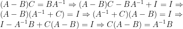
. ?). It is easy to state the problem for elements in a ring, and it seems unlikely that it should be false for rings, given that it is true for real matrices, so let’s try to work on this conjecture:
 , and suppose that
  .
.


 then
then  and
and  the statement is trivial. So instead we assume
  . Remember that right now we are not trying to give a formal proof of anything, but only to get some ideas of what a proof might look like, so we are free to add this “niceness” –assumptions about
 , so they commute and we have:
 and
and 
 then
then  commute. We can’t just use the same trick as before, because we don’t know that


 and
and  as
as